Simulating Bearing Degradation: Why Pure Statistical Noise Fails in Predictive Maintenance
Most synthetic predictive maintenance data relies on unrealistic statistical noise. This post explores why naive noise fails and demonstrates how to generate modeled bearing faults, offering a rigorous benchmark for industrial fault detection.
Every data-driven project in industrial predictive maintenance (PdM) starts with the same hunt for data. Getting telemetry for a healthy motor is easy: you record the historian feed for a week. Getting data for a failing machine is harder. You wait months for a component to break, destroy expensive equipment on a test rig, or train your models on synthetic data.
The problem is that most synthetic data in PdM is statistical noise. To simulate a failing bearing, people inject Gaussian noise or amplify a sine wave. A model trained on that learns to detect unphysical noise, not a mechanical fault.
In this post we generate three vibration series with TSERIZ from the same random seed: a healthy motor, a bearing that degrades by "getting noisier" (Case A), and a bearing with a physically modelled inner-race fault (Case B). Later, a weaker version of that fault (Case C) serves as a stress test. We check that the generator produced what we asked for, then compare how common condition indicators respond. The two degraded series are built so that their overall RMS grows by the same amount. Only one of them contains a fault.
The Physics of a Failing Bearing (Simplified)
When the inner race of a bearing develops surface fatigue, such as a micro-pit or a spall, the bearing does not just get noisier. It develops a specific mechanical signature. Every time a rolling element passes over the pit, it strikes the race like a small hammer. That gives three features to model:
- The fault frequency. The impacts repeat at the Ball Pass Frequency Inner (BPFI). For a 1800 RPM motor (30 Hz shaft) and a bearing with a BPFI multiplier of 5.4, that is 162 Hz. This is the repetition rate of the impacts, not the frequency at which each one rings.
- The impulse shape. Each impact is a second-order underdamped transient: a sharp spike that rings and decays within a few milliseconds. It rings at a structural resonance of the machine, here 600 Hz with a damping ratio of 0.1.
- The noise floor. Real sensors produce white electronic noise and pink mechanical noise. As a bearing wears, the pink component rises.
Generating Three Series with TSERIZ
All three series share the same configuration except for the degradation: 20 seconds sampled at 8192 Hz, a 30 Hz shaft with harmonics at 60 and 90 Hz (0.5, 0.2 and 0.1 g), pink noise with a standard deviation of 0.05 g and white noise of 0.02 g. The first 10 seconds are healthy in all three. Degradation runs from 10 s to 20 s. All three use seed 4242. A weaker variant of Case B, Case C, is introduced later in the article and is run only over seeds 1001 to 1030.
| Series | Between 10 s and 20 s |
|---|---|
| Baseline | Nothing changes. |
| Case A (naive) | Pink noise x1.5 and white noise x9. No impulses. |
| Case B (physics) | Impacts at 162 Hz ringing a 600 Hz resonance (damping ratio 0.1), amplitude 0.1 g growing to 0.5 g. Pink noise x1.5. |
| Case C (weak fault) | Same impacts as Case B, but a constant 0.1 g with no growth. Pink noise x1.5. |
The sampling rate matters. At 2048 Hz, a 600 Hz resonance is rendered with a peak about 6% below the configured amplitude, and the 162 Hz harmonics up to 1 kHz are close to the Nyquist limit. At 8192 Hz the error is under 1%.
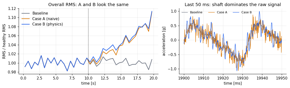
The white-noise gain in Case A (x9) was chosen so that the RMS growth of A and B matches. Over the last two seconds (18 to 20 s, against the healthy first 10 s) the RMS rises 8.6% in Case A and 8.9% in Case B, and by about 11% in both in the final half second. Anything that separates the two is therefore not a matter of overall level.
The healthy baseline
The series in this article were created by importing JSON configurations into TSERIZ, which makes them exactly reproducible (the files are in the repository). The prompts below are the agent route to the same configurations; the exported configuration of each can be compared with the JSON files field by field.
The prompt:
“Simulate 20 seconds of single-channel vibration data in g, sampled at 8192 Hz, with seed 4242, for a motor running at 1800 RPM. Include sinusoidal shaft components at 30 Hz (0.5 g), 60 Hz (0.2 g) and 90 Hz (0.1 g), plus pink mechanical noise with standard deviation 0.05 g and white electronic noise with standard deviation 0.02 g. Set the AR coefficient of both noise components to 0.”
Case A: naive noise degradation
The prompt:
“Simulate 20 seconds of single-channel vibration data in g, sampled at 8192 Hz, with seed 4242, for a motor running at 1800 RPM. Include sinusoidal shaft components at 30 Hz (0.5 g), 60 Hz (0.2 g) and 90 Hz (0.1 g), plus pink mechanical noise with standard deviation 0.05 g and white electronic noise with standard deviation 0.02 g. Set the AR coefficient of both noise components to 0. Between t=10 s and t=20 s, ramp the pink noise amplitude linearly to 1.5 times its starting value and the white noise amplitude linearly to 9 times. Add no transients.”
The video below shows the Case A prompt being entered into the TSERIZ AI agent and the series it produces. The agent turns the plain-English description into a configuration, which can be inspected and exported as JSON, and the series can be downloaded as CSV.
Case B: inner-race fault
The prompt:
“Simulate 20 seconds of single-channel vibration data in g, sampled at 8192 Hz, with seed 4242, for a motor running at 1800 RPM. Include sinusoidal shaft components at 30 Hz (0.5 g), 60 Hz (0.2 g) and 90 Hz (0.1 g), plus pink mechanical noise with standard deviation 0.05 g and white electronic noise with standard deviation 0.02 g. Set the AR coefficient of both noise components to 0. From t=10 s, add an inner-race bearing fault: an underdamped second-order impulse response with natural frequency 600 Hz, damping ratio 0.1 and peak amplitude 0.1 g, repeating 162 times per second. Ramp its amplitude linearly to 5 times (400% growth) at t=20 s. Over the same window, ramp the pink noise linearly to 1.5 times its starting value.”
Case C: weaker version of B
This case is used later as a stress test. It was generated using the same Case B prompt with “constant peak amplitude 0.1 g (no growth)” in place of the amplitude ramp, and keeps the pink-noise ramp.
Checking the Generator Before Trusting It
A synthetic dataset is only useful if it contains what you asked for. Four checks against the exported configuration:
- Shaft lines. Fitted amplitudes are 0.500, 0.201 and 0.100 g, against 0.5, 0.2 and 0.1 g configured.
- Paired design. Because the series share a seed, the first 10 seconds of Case A and Case B are identical to the baseline (maximum difference 0.0). Any difference after 10 s comes from the degradation alone. Real measurements can never give you this.
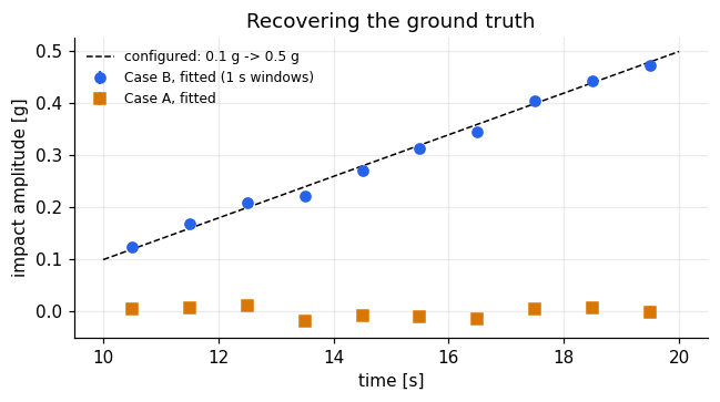
- Fault amplitude. A least-squares fit of the impact train recovers 0.102 g at onset and a growth of 0.039 g/s, against 0.100 g and 0.040 g/s configured. The fit finds nothing in the baseline and nothing in Case A. The formal fit errors understate the true uncertainty because pink noise is correlated, so read the 2% slope difference as agreement.
- Pink-noise ramp. Comparing each degraded series with the baseline isolates the extra pink noise. Its scale grows from 1 to 1.5 as configured: in each one-second window the measured excess matches the configured value to within 0.01 (0.475 against 0.475 in the last window).
What the Fault Looks Like
Before any analysis, here is the data itself. TSERIZ returns each series as a two-column CSV with a timestamp and a vibration value. The three series share a seed and a configuration, so they are identical up to 10 s. From the next row, Case B starts to ring from its first impact, while Case A differs from the baseline only in the sixth decimal because its noise ramp has just begun. Figure 2 shows the rows around the onset and, below them, each series minus the baseline: just after the onset (left), where Case B's impacts repeat every 6.17 ms and Case A is still flat, and at the end of the record (right), where Case A is broadband noise and Case B is a train of bursts.
In the raw signal the shaft dominates (Figure 3, right). The overall RMS of the two degraded series rises together (Figure 3, left), which is the problem: from RMS alone, A and B are the same failure.
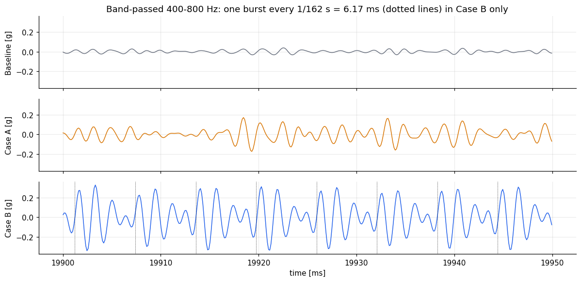
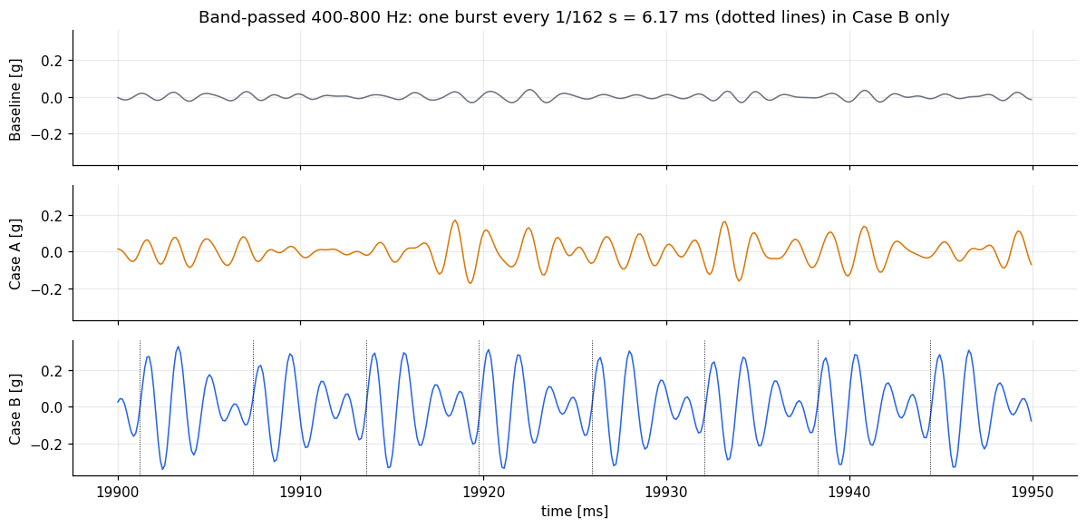
Band-pass the signal around the resonance (400 to 800 Hz) and the fault appears. In Case B there is one burst every 6.17 ms, with a peak of about 0.3 g near the end of the record. In Case A there is only a louder noise floor.
Figure 4: 400 to 800 Hz band, 19.90 to 19.95 s. Dotted lines in the Case B panel mark the configured impact times (162 Hz)
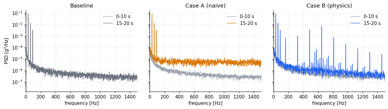
In the spectrum, Case A lifts the whole noise floor. Case B adds a comb of lines at multiples of 162 Hz, but its energy is small compared with the shaft, which is why the RMS barely moves.
Figure 5: power spectral density, 0 to 1500 Hz, 0 to 10 s against 15 to 20 s.
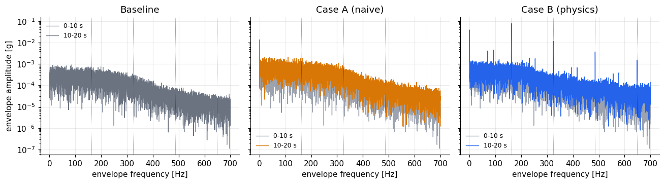
The envelope spectrum, the spectrum of the amplitude envelope of the resonance band, shows the repetition rate directly. In Case B the line at 162 Hz stands 173 times above the surrounding envelope floor, with harmonics at 324 Hz (74 times) and 486 Hz (49 times). In the baseline and in Case A the same ratio is below 3, which is the level of the noise itself.
Figure 6: envelope spectrum of the 400 to 800 Hz band, 0 to 10 s against 10 to 20 s. Dotted lines at 162 Hz and its harmonics.

Generating 90 More Series with the TSERIZ API
One series per case shows that a detector can find a fault. It does not show how much the detection delay depends on the particular noise realisation. For that, the same configuration has to run many times with only the random seed changed, and that is where a programmatic API earns its place. We designed each case once in the TSERIZ UI, exported its configuration as JSON, and used the REST API to generate 30 seeds (1001 to 1030) of each of Cases A, B and C: 90 series of 163,841 points each, which feed the Monte Carlo results below.
- The seed is a request field, separate from the configuration. The configuration stays untouched, and the same configuration and seed always return the same series.
- Check before you spend. A free validation call checks a configuration and reports the estimated number of points, and quota and capability endpoints let a script confirm that a batch fits the plan limits before it starts.
- Prove that the script matches the UI. Before generating anything new, we regenerated seed 4242 through the API and compared it with the CSVs downloaded from the UI. Every value matched, in both cases.
- The data comes back in the response, so there is no separate download step. Each run returns an id, a status and the seed, and a manifest saved with the CSVs records them for an audit trail.
- A well-behaved batch client honours rate limits, backs off when asked, and skips files that already exist, so an interrupted batch can be resumed.
Each series took about two seconds to generate, so the 60 series for Cases A and B took around two minutes, and every series then passed the configuration check described above.
Detecting It: RMS Against the Envelope Line
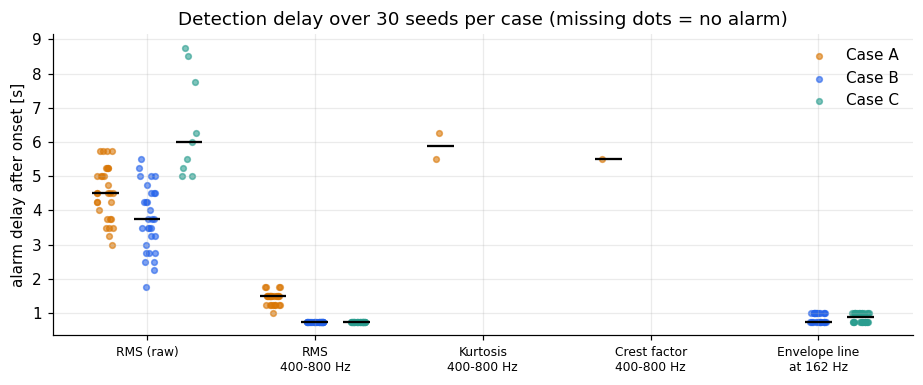
Because the onset is known, detectors can be scored by how late they alarm. Each indicator is computed in one-second windows with a 0.25 s step. The alarm threshold is the mean plus four standard deviations of the indicator over the healthy first 10 seconds, and an alarm needs three consecutive windows above it. The delay runs from the onset to the end of the third window. The table gives the median delay over 30 seeds per case (seeds 1001 to 1030), with the 10th to 90th percentile in brackets and the number of series in which the indicator raised an alarm. Each series sets its own threshold. Delays come in steps of 0.25 s, and 0.75 s is the shortest the rule can give. On healthy data held out from the calibration (threshold from 0 to 6 s, rule applied to 6 to 10 s), 1 of the 30 healthy records raised a false alarm for the band RMS, 1 for the envelope line and 2 for the crest factor, and none did for overall RMS or kurtosis. A seed's healthy first 10 seconds are the same in every case, so these are 30 records, not 90.
| Indicator | Case A: median delay (10th to 90th percentile), alarms | Case B: median delay (10th to 90th percentile), alarms | Case C: median delay (10th to 90th percentile), alarms |
|---|---|---|---|
| Overall RMS | 4.50 s (3.50 to 5.75), 30 of 30 | 3.75 s (2.50 to 5.00), 30 of 30 | 6.00 s (5.00 to 8.55), 9 of 30 |
| RMS, 400 to 800 Hz | 1.50 s (1.25 to 1.75), 30 of 30 | 0.75 s (0.75 to 0.75), 30 of 30 | 0.75 s (0.75 to 0.75), 30 of 30 |
| Envelope line at 162 Hz | 0 of 30 | 0.75 s (0.75 to 1.00), 30 of 30 | 0.88 s (0.75 to 1.00), 30 of 30 |
| Kurtosis, 400 to 800 Hz | 2 of 30 | 0 of 30 | 0 of 30 |
| Crest factor, 400 to 800 Hz | 1 of 30 | 0 of 30 | 0 of 30 |
Figure 7: each indicator in one-second windows (0.25 s step) for the baseline and Cases A and B, seed 4242. Dashed lines mark the alarm thresholds (mean plus four standard deviations of the healthy windows); the dotted line marks the onset at 10 s.
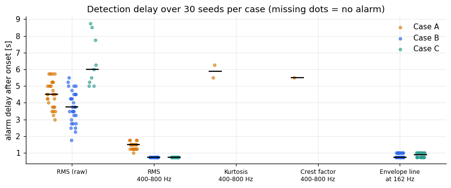
- Overall RMS alarms after a median of 3.75 s in Case B and 4.5 s in Case A, and the delay varies by about 2.5 s between seeds. The two cases overlap, so RMS cannot tell A from B. That follows from how the cases were built. For the weaker Case C it alarms in only 9 of 30 series, after a median of 6 s.
- RMS in the resonance band is faster (0.75 s in Case B, 1.5 s in Case A), but it alarms in every Case A series too. It reacts to any extra energy in the band, and how well it separates A from B here depends on how much energy each case happens to add.
- The envelope line at 162 Hz alarms in all 30 Case B series after 0.75 to 1.0 s, which is the shortest delay the rule allows, and in none of the Case A series. It is the only indicator here that says what kind of degradation is happening.
- Kurtosis and crest factor almost never alarm (2 and 1 of the 30 Case A series, none in Case B). In the seed 4242 series (Figure 7), kurtosis spikes for two windows that straddle the onset (half healthy, half faulty), then falls below its healthy value (2.3 against 3.0). With 162 impacts per second and a decay time of 2.6 ms, the bursts overlap and the band signal looks like a modulated sine, not a set of isolated spikes. Impulsiveness indicators suit slow faults with well-separated impacts. The fault's physical parameters decide which indicator works.
What Each Kind of Degradation Teaches a Detector
To see what a detector learns from each kind of degradation, we trained a logistic regression on window features (overall RMS, band RMS, kurtosis and crest factor) to separate healthy windows from fully degraded ones. Each model was trained on 15 seeds of one case and tested on the other 15 seeds, of the same case and of the other case.
Trained on Case A, the model works on Case A (AUC 0.999, 93% of degraded windows flagged) and on Case B (AUC 1.000, 100% flagged). The naive detector catches this fault, because by the end of the record the fault has added a lot of energy to the resonance band. Trained on Case B, the model works on Case B (AUC 1.000, 100% flagged) but misses Case A (AUC 0.67, 3% flagged). A detector trained on the physical fault does not mistake a noisier machine for a bearing fault. A detector trained on noise flags both and cannot say which one it found. Adding the envelope line as a feature changes none of this, since the other features already separate the classes at these fault amplitudes.
This is weaker than the claim that naive data produces detectors that miss real faults. What it shows is that data from Case A alone cannot tell you whether a detector is specific, and that a detector trained on it is not tested against the signature that matters. Case C, below, tests whether it still works when the fault is small.
Stress test: Case C, a fault that does not grow
A fair objection is that Case B's fault is large by the end of the record. Case C is Case B without the amplitude ramp: the same impacts at 162 Hz ringing the 600 Hz resonance, the same pink-noise growth, but a constant 0.1 g from 10 s to 20 s. It is Case B at its first impact, and it never gets worse. We generated it for the same 30 seeds. Its first 10 seconds are identical to the other cases for the same seed, and all 30 series pass the configuration checks (the growth check was replaced by one that tests that the burst level matches the model and stays constant).
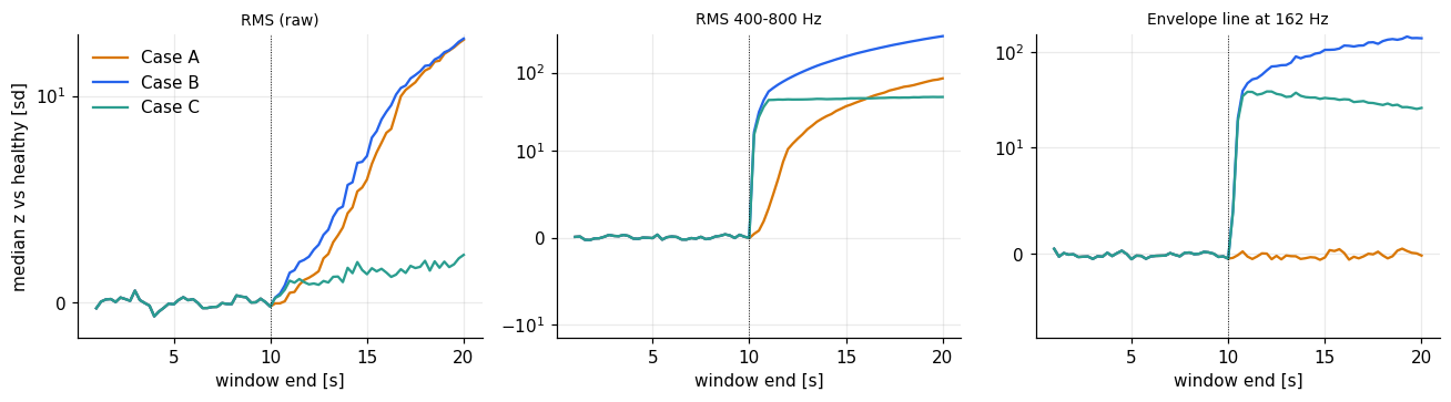
Overall RMS barely sees this fault. After onset its median sits 1.5 healthy standard deviations above the healthy level, against 7.1 for Case A and 8.3 for Case B, and it raises an alarm in only 9 of 30 series, after a median of 6.0 s (5.0 to 8.6). The band RMS alarms in all 30 series after 0.75 s, and the envelope line at 162 Hz in all 30 after a median of 0.88 s (0.75 to 1.00).
The cross-test gives a more careful answer than we expected. The detector trained on Case A, which only ever saw louder noise, flags 100% of the degraded Case C windows (AUC 1.000, no false positives on healthy windows). The reason is the band RMS: Case C adds about as much energy to the 400 to 800 Hz band as Case A does (median 47 against 41 healthy standard deviations after onset), even though its overall RMS hardly moves. With overall RMS alone the picture changes: trained on Case A it flags 41% of degraded Case C windows, and trained on Case C it flags 73% with 27% false positives (AUC 0.80). In the other direction, a model trained on Case C flags 60% of Case A windows (AUC 0.92) and all of Case B, and a model trained on Case B flags 90% of Case C and 3% of Case A.
So the claim stays in its weaker form. These data do not show that a detector trained on naive degradation misses a real fault, even a small one, as long as it looks at the resonance band. What they show is that the two cases differ in the one thing the naive detector was never given. Case A and Case C both raise the band RMS, but only Case C raises the envelope line at 162 Hz (median 32 healthy standard deviations after onset, against -0.2 for Case A; the line separates the two cases perfectly at the end of the record, AUC 1.00). A detector trained on Case A flags the fault but cannot say it found a bearing fault, and a fault that overall RMS alarms on late, and in fewer than a third of the series, is caught within a second by an indicator built from the physics.
Figure 9: median over 30 seeds of overall RMS, band RMS and envelope line at 162 Hz, in healthy standard deviations (symmetric log scale), for Cases A, B and C. Dotted line: onset at 10 s. Case C's envelope line drifts down slowly as the pink-noise floor rises.
Limits and What To Use It For
Synthetic data tests whether a method can find a fault of known form. It does not replace validation on measured bearings. This fault is idealised: constant speed, one resonance, perfectly periodic impacts (rounded to the nearest sample, so the timing is exact within half a sample), and no slip between rolling elements and race. Real bearings have jitter that smears the envelope lines, so expect real detection delays to be longer.
Within those limits it is useful for questions you cannot answer with a handful of real failures: what sampling rate and band you need to see the fault, how alarm thresholds trade delay against false alarms, which indicators separate fault types, and how much lead time a method gives before a given damage level.
Try It Yourself
The code, configurations and sample data are in our public GitHub repository, synthetic-bearing-fault-benchmarks: https://github.com/deuxlatis/synthetic-bearing-fault-benchmarks. It contains the Python notebook that produced the figures and numbers in this post, the exported TSERIZ configurations for the baseline and Cases A, B and C, the script that checks a series against its configuration, and sample datasets of up to 50,000 points per series, small enough to generate on the free TSERIZ tier. The sample datasets are for trying your own detectors. They are shorter than the full series, so they do not reproduce the numbers in this post. The full 20-second series have 163,841 points each; to reproduce the exact numbers, regenerate them from the configurations in the repository (seed 4242, and seeds 1001 to 1030 for the Monte Carlo runs).
To change the RPM or the BPFI multiplier, or to add missing-data dropouts to stress-test an ingestion pipeline, adapt the prompts above with a free account at tseriz.com.